Sources and boundaries
Time signals and incident fields
Time signals provide their first and second derivatives analytically, which is needed by the dipole current and its reference field. Plane waves are solutions in a homogeneous, lossless, nondispersive background material. They can be used as initial conditions, boundary data or TF/SF excitation. Superposition adds the physical fields and retains one set of default material parameters.
MaxwellTrixi.GaussianPulse — Type
GaussianPulse(width; delay = 0)Time signal $s(t) = \exp(-((t - t_0) / w)^2)$ with width $w$ and delay $t_0$. Callable as signal(t); signal_derivative and signal_second_derivative give $\dot s$ and $\ddot s$.
MaxwellTrixi.ModulatedGaussianPulse — Type
ModulatedGaussianPulse(frequency, width; delay = 0, phase = 0)Time signal $s(t) = \exp(-((t - t_0) / w)^2) \sin(2 \pi f (t - t_0) + \phi)$. Two signals with phases $0$ and $\pi / 2$ on orthogonal polarizations give a circularly polarized PlaneWave.
MaxwellTrixi.signal_derivative — Function
signal_derivative(signal, t)
signal_second_derivative(signal, t)
First and second time derivative of a signal.
MaxwellTrixi.signal_second_derivative — Function
signal_derivative(signal, t)
signal_second_derivative(signal, t)
First and second time derivative of a signal.
MaxwellTrixi.AbstractIncidentField — Type
AbstractIncidentFieldAnalytic free-space solution field(x, t, equations) in the background material of the equations, returned with the default material components. Usable as initial condition, in BoundaryConditionIncidentField and in TotalFieldScatteredField. Two fields are superposed with +.
MaxwellTrixi.PlaneWave — Type
PlaneWave(direction, polarization, signal)Plane wave $E = s(t - \hat k \cdot x / c) \, e$, $H = Y \, \hat k \times E$ with the unit propagation direction $\hat k$, the polarization vector $e$ (amplitude included, orthogonal to $\hat k$) and a time signal such as GaussianPulse. Requires a homogeneous, lossless, nondispersive background material; $c$ and $Y$ are taken from the equations object.
MaxwellTrixi.initial_condition_zero — Function
initial_condition_zero(x, t, equations::MaxwellEquations3D)Zero fields with the default material of the equations.
julia> using MaxwellTrixi

julia> pulse = GaussianPulse(0.4; delay = 1.4);

julia> pulse(1.4), signal_derivative(pulse, 1.4)
(1.0, -0.0)
Periodic plane wave example
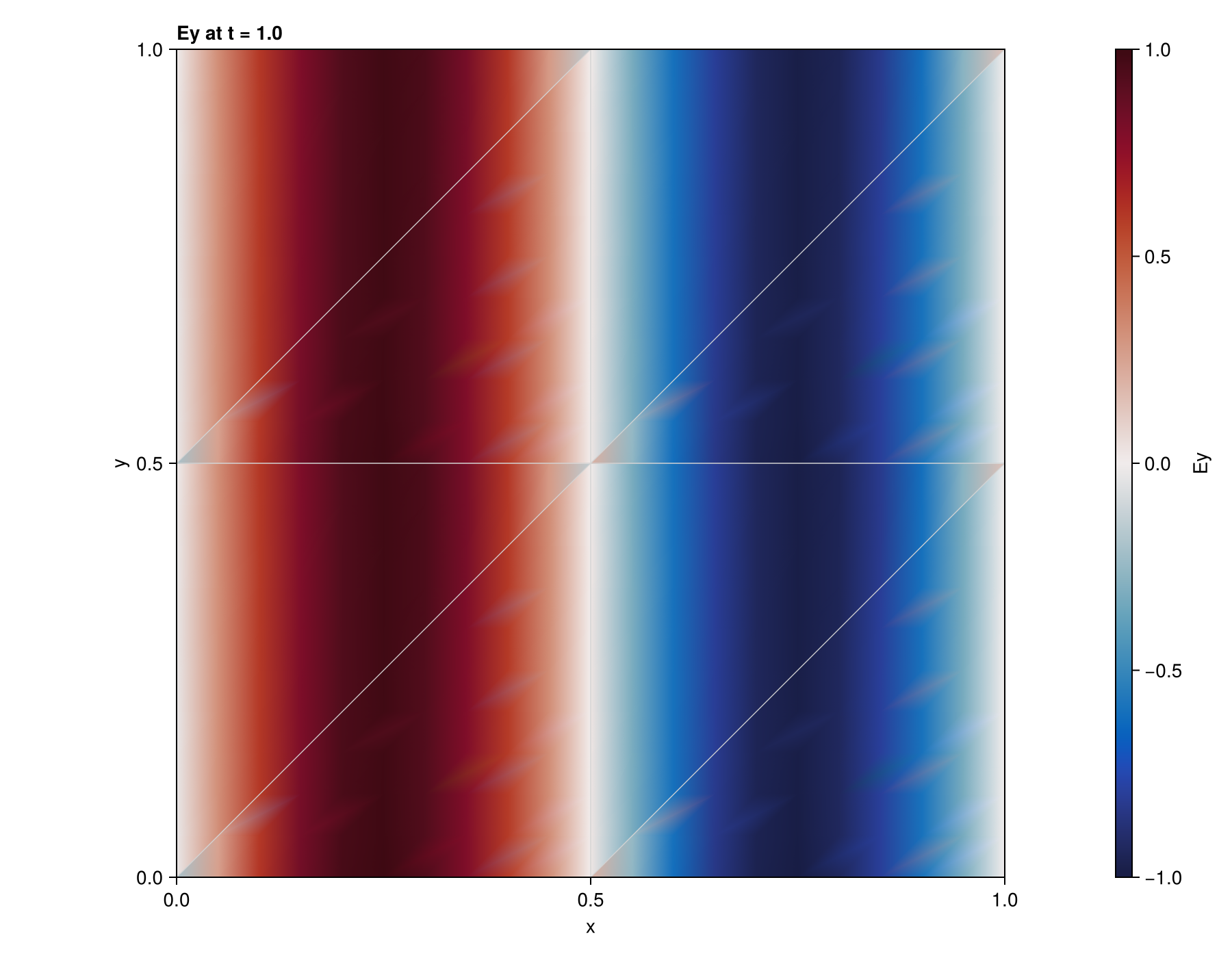
This periodic-domain example shows a plane wave propagating through the tetrahedral mesh.
Regularized electric dipole
The dipole injects an impressed electric current, so it enters the electric field equation with a minus sign. Its spatial Gaussian has unit integral over all space. ProjectedSourceTerms helps retain that strength on DGSEM meshes. The analytical exterior reference assumes a homogeneous, lossless, nondispersive background and accounts for Gaussian regularization of a Gaussian time pulse. Compare it outside the source region and before boundary reflections return.
MaxwellTrixi.HertzianDipole — Type
HertzianDipole(position, moment, width, signal)Electric dipole $p(t) = s(t) \, p_0$ at position with moment $p_0$ and time signal $s$, regularized in space over $G_w(x) = \exp(-|x - x_0|^2 / w^2) / (\pi^{3/2} w^3)$. Passed as source_terms it drives Ampère's law with the current density
\[J_{\mathrm{src}}(x,t) = \dot s(t)\,p_0\, \frac{\exp(-|x-x_0|^2/w^2)}{\pi^{3/2}w^3}\]
and adds the Ohmic loss of source_terms_conductivity. The exact field of the point dipole is HertzianDipoleField.
MaxwellTrixi.HertzianDipoleField — Type
HertzianDipoleField(position, moment, signal)
HertzianDipoleField(dipole::HertzianDipole, equations)
Exact field of the point dipole $p(t) = s(t) \, p_0$ in a homogeneous, lossless, nondispersive background material, with $R = |x - x_0|$, $\hat r = (x - x_0) / R$ and all moments taken at the retarded time $t - R / c$:
\[E = \frac{1}{4 \pi \epsilon} \left( \frac{3 \hat r (\hat r \cdot p) - p}{R^3} + \frac{3 \hat r (\hat r \cdot \dot p) - \dot p}{c R^2} + \frac{\hat r \times (\hat r \times \ddot p)}{c^2 R} \right), \quad H = \frac{1}{4 \pi} \left( \frac{\dot p \times \hat r}{R^2} + \frac{\ddot p \times \hat r}{c R} \right).\]
Outside the source region $R \gg w$ the regularized HertzianDipole radiates like a point dipole whose signal is $s$ convolved with the line-of-sight profile of $G_w$, a Gaussian of width $w / c$. For a GaussianPulse of width $a$ this is a Gaussian pulse of width $\sqrt{a^2 + (w/c)^2}$ with the moment scaled by $a / \sqrt{a^2 + (w/c)^2}$, which the second constructor applies.
Dipole on tetrahedra example
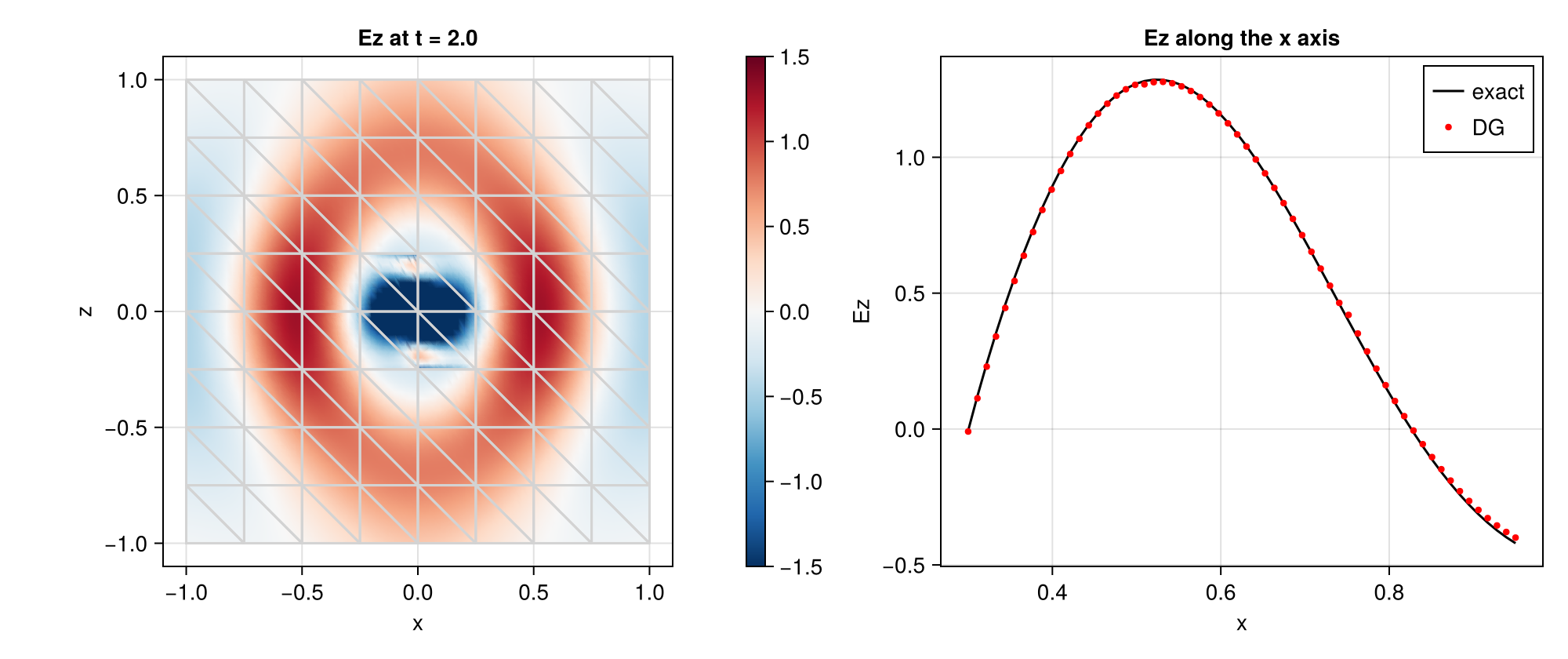
The field slice accompanies a numerical-versus-analytical line probe. Source regularization and spatial resolution both affect agreement near the source.
Total-field/scattered-field injection
TF/SF injection confines the incident wave to a chosen region. With no scatterer, the exterior should remain close to zero; this is a useful leakage test.
MaxwellTrixi.TotalFieldScatteredField — Type
TotalFieldScatteredField(incident_field, mesh::DGMultiMesh, is_total_field)Total-field/scattered-field interface on all interior faces between elements whose centroids is_total_field(x) classifies differently. Used as a value of boundary_conditions, it recomputes the interface flux on these faces with the incident field added to the neighbor state seen from the total-field side and subtracted on the scattered-field side, so the incident wave exists only in the total-field region. For the physical fields,
\[u_{\mathrm{stored}} = \begin{cases} u_{\mathrm{inc}} + u_{\mathrm{scat}}, & x \in \Omega_{\mathrm{TF}}, \\ u_{\mathrm{scat}}, & x \notin \Omega_{\mathrm{TF}}. \end{cases}\]
Outside the total-field region, add the incident field to reconstruct the total field. The incident field must be a free-space solution in the background material, which has to fill the interface faces. Start from initial_condition_zero with a delayed signal, or with the incident field if it is still outside the domain.
MaxwellTrixi.FluxTotalFieldScatteredField — Type
FluxTotalFieldScatteredField(surface_flux, incident_field, is_total_field)Surface flux for DGSEM on P4estMesh and T8codeMesh that applies the total-field/scattered-field correction of TotalFieldScatteredField on the interior faces between elements whose centroids is_total_field(x) classifies differently, and behaves like surface_flux everywhere else. The faces are marked on the first right-hand side evaluation and again after every mesh adaptation; the interface must not cross mortars, so both sides of it have to be refined equally.
On DGMulti, TotalFieldScatteredField is installed through boundary_conditions; it recomputes selected interior face fluxes during the boundary-flux stage, where time and face coordinates are available. On P4est and T8code DGSEM, FluxTotalFieldScatteredField wraps the surface flux and records the current stage time in a specialized RHS hook.
The TF/SF surface must follow element faces in the background medium. The DGSEM implementation rejects a TF/SF surface crossing a mortar; refine both sides of that surface equally. Its marks are rebuilt when the element, interface or mortar counts change. Start with a delayed incident pulse and a consistent initial state; injection does not repair inconsistent initial data.
TF/SF in free space example
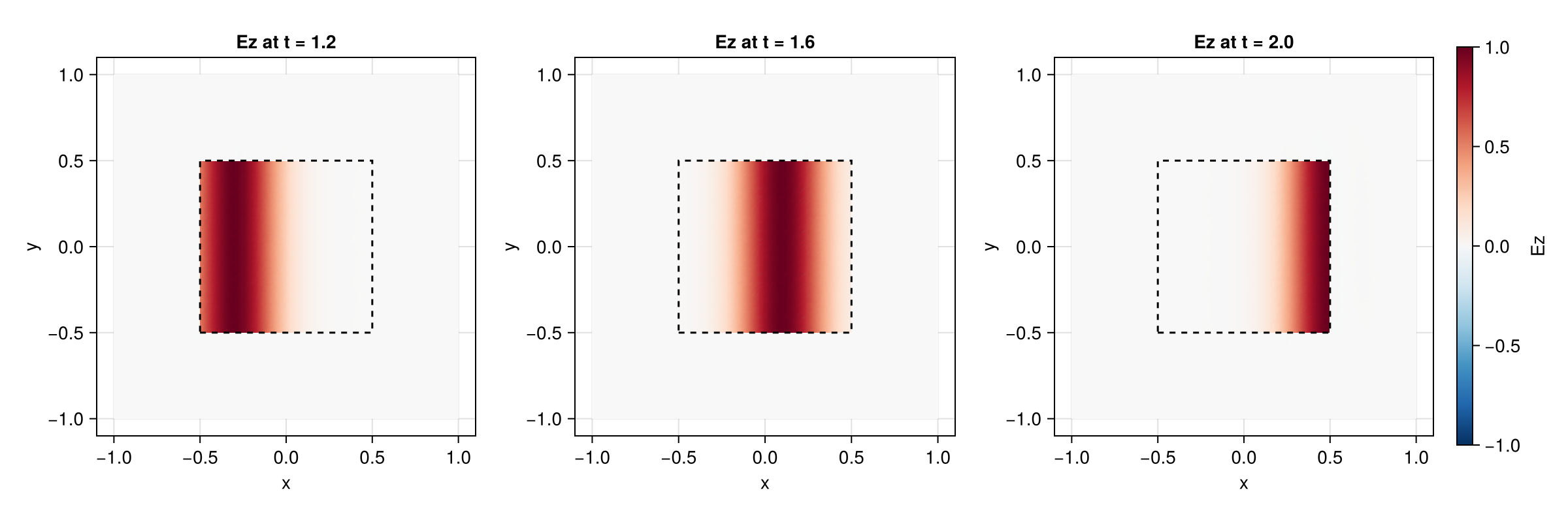
With no scatterer, the stored field outside the dashed TF box stays close to zero. This visualizes cancellation of the incident field on the scattered-field side.
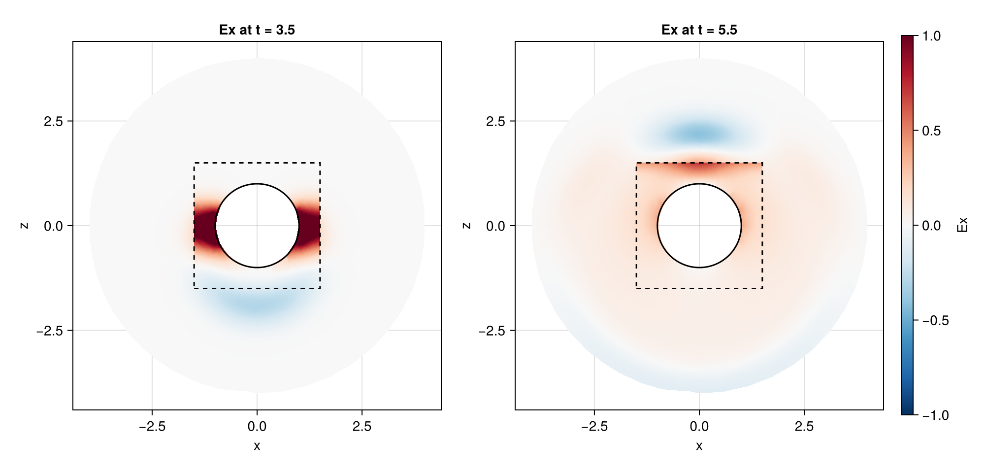
PEC sphere with TF/SF example
The PEC sphere reflects the injected pulse. The stored field is total inside the dashed box and scattered outside.
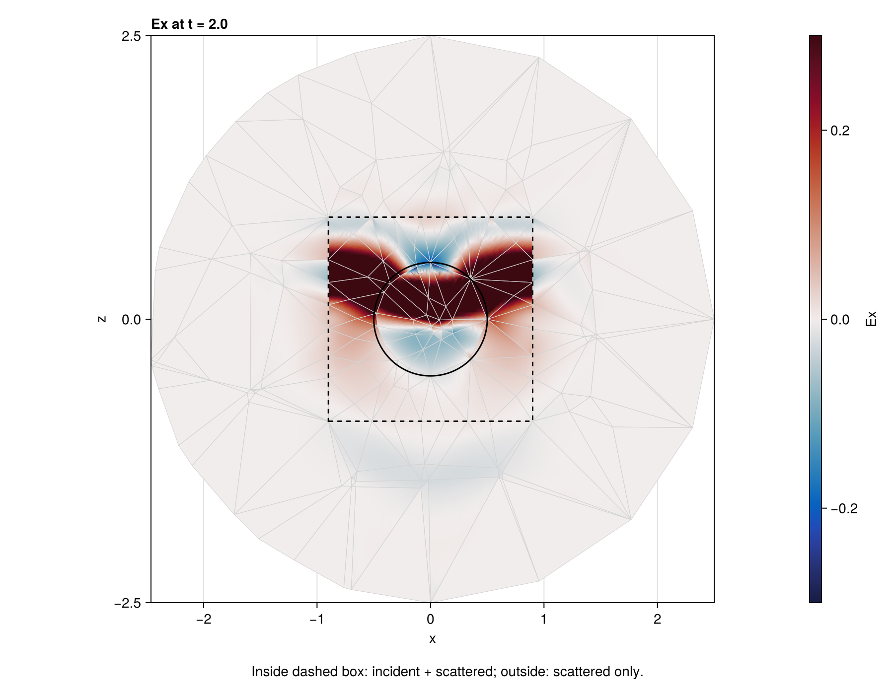
Dielectric TF/SF scattering example
The dielectric sphere scatters the injected pulse. This slice uses affine tetrahedra; the numerical Mie example also supports curved geometry.
Physical boundary conditions
For outward unit normal $n$, the ideal conditions are
\[n\times E=0\quad\text{(PEC)},\qquad n\times H=0\quad\text{(PMC)}.\]
The implementation supplies reflected exterior fields to the numerical flux. Only tangential components enter the Maxwell normal flux. Silver–Mueller sets the incoming characteristic to zero; it is exact for an outgoing plane wave at normal incidence and approximate for oblique waves. Prescribed incident fields enter as exterior states of the scheme's surface flux; with flux_upwind only their incoming characteristic enters the domain.
MaxwellTrixi.boundary_condition_perfect_electric_conductor — Constant
boundary_condition_perfect_electric_conductor = BoundaryConditionPerfectElectricConductor()Perfect electric conductor: exterior state (-E, H) with the interior material, evaluated with the surface flux of the scheme.
MaxwellTrixi.boundary_condition_perfect_magnetic_conductor — Constant
boundary_condition_perfect_magnetic_conductor = BoundaryConditionPerfectMagneticConductor()Perfect magnetic conductor: exterior state (E, -H) with the interior material, evaluated with the surface flux of the scheme.
MaxwellTrixi.boundary_condition_silver_mueller — Constant
boundary_condition_silver_mueller = BoundaryConditionSilverMueller()First-order absorbing boundary: flux_upwind against an exterior state with zero fields and the interior material, independent of the surface flux of the scheme. Exact for normal incidence only.
MaxwellTrixi.BoundaryConditionIncidentField — Type
BoundaryConditionIncidentField(incident_field)Exterior fields incident_field(x, t, equations) on a boundary face, combined with the interior material. With flux_upwind only the incoming characteristic of the incident field enters the domain.
Uniaxial perfectly matched layer
UPML adds local damping and six auxiliary unknowns. Its profile vanishes in the physical region and grows towards the outer boundary. The directional damping rates $\sigma_x,\sigma_y,\sigma_z$ below are PML parameters, distinct from the material's physical Ohmic conductivity $\sigma$.
MaxwellTrixi.PMLProfile — Type
PMLProfile(coordinates_min, coordinates_max, thickness;
           order = 3, reflection = 1e-6, impedance = 1.0)
Damping profile of a uniaxial perfectly matched layer filling the shell of the given thickness inside the box coordinates_min, coordinates_max, the same values as passed to DGMultiMesh. Along each axis $\sigma_i(x) = \sigma_\mathrm{max} (d_i / \mathrm{thickness})^\mathrm{order}$ with the depth $d_i$ into the layer, zero in the physical region. The default $\sigma_\mathrm{max} = (\mathrm{order} + 1) \ln(1 / \mathrm{reflection}) / (2 Z \, \mathrm{thickness})$ targets the given normal-incidence reflection of the layer terminated by boundary_condition_silver_mueller; pass sigma_max to override it.
MaxwellTrixi.SourceTermsPML — Type
SourceTermsPML(profile)Source term of the uniaxial perfectly matched layer with auxiliary differential equations (Busch, König, Niegemann 2011, eq. 38). With the damping $\sigma = (\sigma_x, \sigma_y, \sigma_z)$ of the profile at the node and cyclic indices $(i,j,k)$, define $a_i = \sigma_j + \sigma_k - \sigma_i$ and $b_i = (\sigma_i - \sigma_j)(\sigma_i - \sigma_k)$. The added field sources and auxiliary equations are
\[\begin{aligned} (s_E)_i &= -a_i E_i - p_i / \epsilon, & \partial_t p_i &= b_i \epsilon E_i - \sigma_i p_i, \\ (s_H)_i &= -a_i H_i - q_i / \mu, & \partial_t q_i &= b_i \mu H_i - \sigma_i q_i. \end{aligned}\]
The directional PML damping rates are distinct from the physical Ohmic conductivity of the material. Requires MaxwellEquations3D with UPML(); the layer must continue the background material of the adjacent physical region.
MaxwellTrixi.CombinedSourceTerms — Type
CombinedSourceTerms(terms...)Sum of several source terms term(u, x, t, equations), for example SourceTermsPML together with a HertzianDipole.
The layer must continue the adjacent background material. The examples combine its source with the dipole and terminate the outer boundary with Silver–Mueller. test/test_dgmulti_3d.jl and test/test_dgsem_3d.jl compare residual reflection or remaining energy with and without PML.
PML comparison example
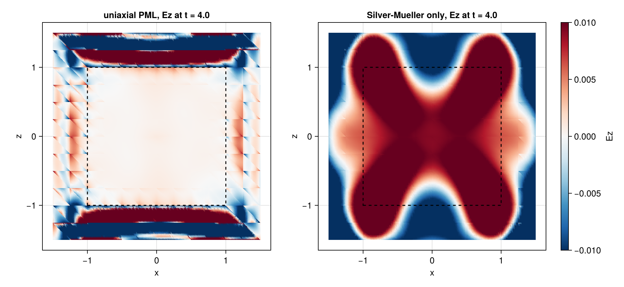
The side-by-side comparison shows UPML and Silver–Mueller alone. Both use the same narrow color scale. The stronger outgoing pulse saturates it, making smaller late reflections visible.