Equations and materials
Curl equations and normalization
MaxwellEquations3D defines the physical fields and the optional state components. In the physical region, the electric-field equation can include Ohmic loss, an impressed current and polarization currents. The magnetic field is non-dispersive in the implemented material models.
MaxwellTrixi.MaxwellEquations3D — Type
MaxwellEquations3D(material = Homogeneous(), absorber = NoPML();
                   epsilon = 1.0, mu = one(epsilon), sigma = zero(epsilon),
                   drude = (), lorentz = ())
MaxwellEquations3D(UPML(); kwargs...)
Maxwell's curl equations for the fields $(E, H)$ in a linear medium. In the physical region, with an impressed current $J_{\mathrm{src}}$ and optional polarization currents $J_k$, the combined model is
\[\begin{aligned} \epsilon_\infty \partial_t E &= \nabla \times H - \sigma E - J_{\mathrm{src}} - \sum_k J_k, \\ \mu \partial_t H &= -\nabla \times E. \end{aligned}\]
For a nondispersive medium $\epsilon_\infty = \epsilon$ and the sum is empty. The flux supplies the curl terms; conductivity, impressed currents and material poles require the corresponding source terms in the semidiscretization. PML adds the local terms described by SourceTermsPML. Units are normalized: epsilon and mu are relative values, the vacuum speed of light and impedance are one, and a conductivity $\sigma$ in SI units becomes $\sigma Z_0 L$ for the length unit $L$.
The material model is a type parameter. With Homogeneous, the default, the state is (Ex, Ey, Ez, Hx, Hy, Hz) and the material lives in the struct. With Heterogeneous the state carries the passive components epsilon, mu, sigma per node; they have zero flux and are set per element with set_materials!, the struct values being the defaults written by initial conditions. sigma only acts when source_terms_conductivity is passed as the source term of the semidiscretization.
With UPML the state additionally carries the auxiliary fields (px, py, pz, qx, qy, qz) of the uniaxial perfectly matched layer, with zero flux and zero initial value. They are driven by SourceTermsPML inside the layer and stay zero elsewhere.
Dispersive media follow from the drude and lorentz tuples of DrudePoles and LorentzPoles; epsilon is then the high-frequency permittivity $\epsilon_\infty$. Each Drude pole adds a polarization current (Jx, Jy, Jz), each Lorentz pole a polarization and its current (Px, Py, Pz, Jx, Jy, Jz), all with zero flux and zero initial value, driven by source_terms_dispersive. With Homogeneous the poles describe the medium; with Heterogeneous the state also carries the pole parameters per node, set with set_materials!, and the poles of the struct are their defaults.
Choose a length scale $L$ and electric-field scale $E_0$. With SI quantities on the right, the dimensionless variables are
\[x = x_{\rm SI}/L,\qquad t = c_0 t_{\rm SI}/L,\qquad E = E_{\rm SI}/E_0,\qquad H = Z_0 H_{\rm SI}/E_0.\]
Thus vacuum has $\epsilon=\mu=c=Z=1$. In a nondispersive material,
\[c=(\epsilon\mu)^{-1/2},\qquad Z=(\mu/\epsilon)^{1/2},\qquad Y=1/Z.\]
Conductivity becomes $\sigma=\sigma_{\rm SI}Z_0L$ and an angular frequency becomes $\omega=\omega_{\rm SI}L/c_0$. Ordinary frequencies used by signals and transforms obey $\omega=2\pi f$.
The code evolves the curl system without an additional charge-density equation or divergence-cleaning field. The diagnostics measure elementwise divergences of $E$ and $H$; they do not enforce the Gauss constraints.
PEC cavity example
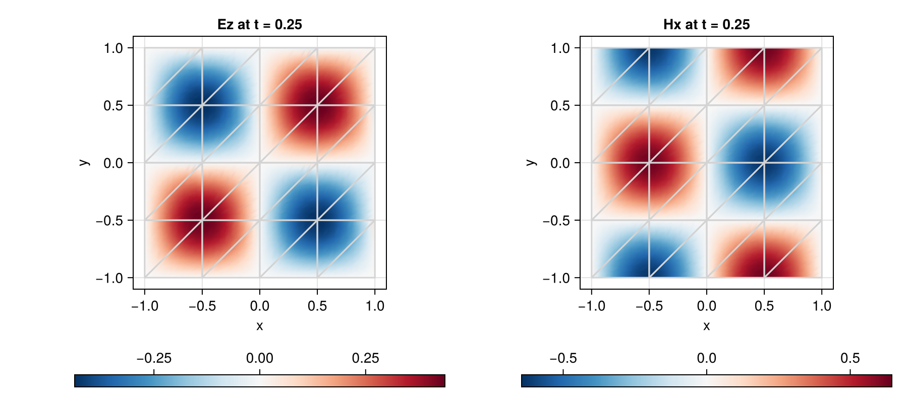
The cavity example shows the coupled electric and magnetic TM-mode fields. Its analytical reference is discussed under Diagnostics and validation.
State layout and static materials
The state starts with (Ex, Ey, Ez, Hx, Hy, Hz). Its remaining blocks are:
| Model option | Additional components |
|---|---|
Heterogeneous() | epsilon, mu, sigma, then the parameters of each pole |
| Each Drude pole | Three polarization-current components |
| Each Lorentz pole | Three polarization and three current components |
UPML() | Six auxiliary components (px, py, pz, qx, qy, qz) |
Homogeneous() reads material parameters from the equations object. Heterogeneous() reads them from the state. They have zero flux and zero source, so their values remain constant in time on a fixed mesh. set_materials! assigns the same material to every node of an element; material interfaces must therefore follow element faces. These passive parameters are distinct from the dynamical polarization and PML components, which have zero flux but nonzero sources.
MaxwellTrixi.Material — Type
Material(; epsilon = 1.0, mu = one(epsilon), sigma = zero(epsilon),
         drude = (), lorentz = ())
Relative permittivity, relative permeability and normalized conductivity of a linear medium, assigned per element with set_materials!. A dispersive medium adds tuples of DrudePoles and LorentzPoles, with epsilon the high-frequency permittivity $\epsilon_\infty$; it needs equations with at least as many poles of each kind, the remaining poles of the element are inactive.
MaxwellTrixi.set_materials! — Function
set_materials!(u_ode, semi, material_at)
set_materials!(u_ode, semi, element_groups, materials::AbstractDict)
Write the material into the passive components of every node of a MaxwellEquations3D{Heterogeneous} state, element by element. The first form evaluates material_at(x) at the element centroid, the second looks up materials[element_groups[element]], for example with the groups of an ImportedMesh. Both return a Material per element. Call after semidiscretize on ode.u0.
MaxwellTrixi.permittivity — Function
permittivity(u, equations), permeability(u, equations), conductivity(u, equations)
impedance(u, equations), admittance(u, equations), speed_of_light(u, equations)
Material at a node: struct fields for Homogeneous, read from the state for Heterogeneous. The one-argument forms exist for Homogeneous only.
Fresnel interface example
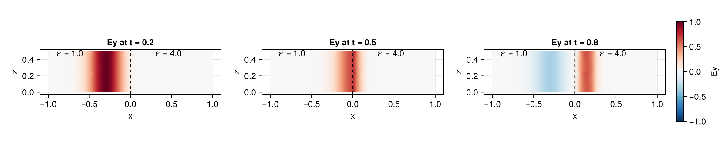
The pulse splits into reflected and transmitted waves at the material interface. The dashed line marks the permittivity jump.
Dielectric sphere example
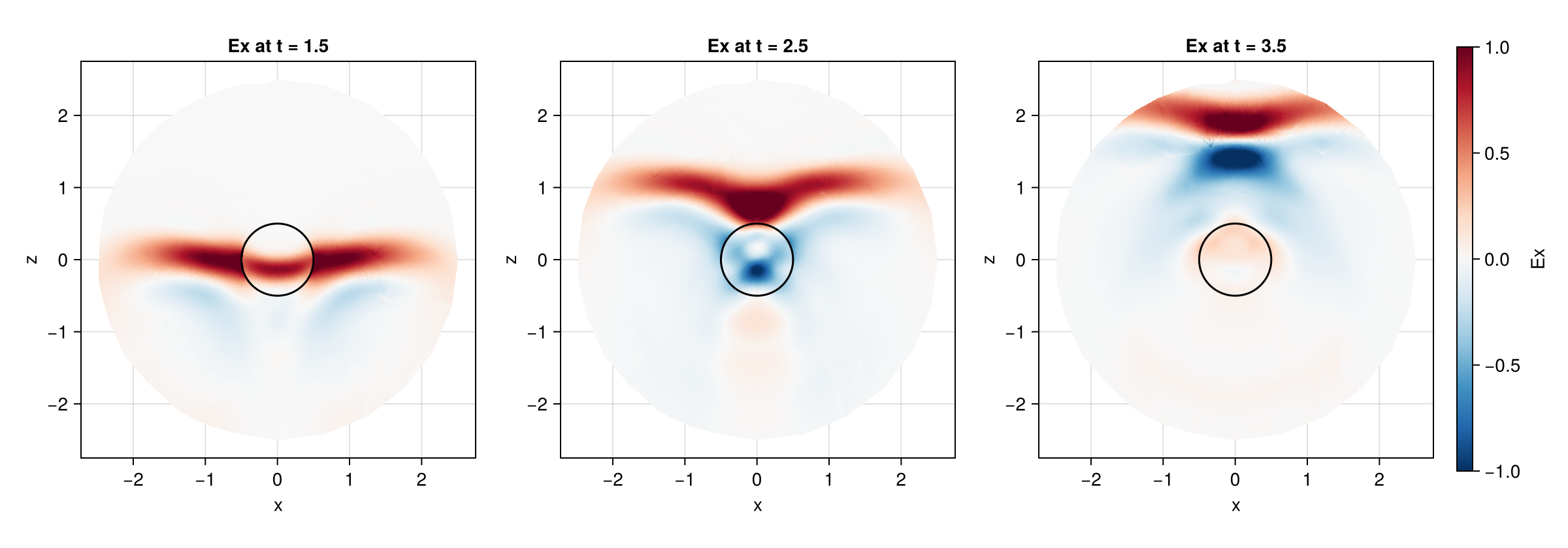
A plane-wave pulse interacts with a dielectric sphere. The outline marks its material interface.
Conductivity and dispersion
epsilon denotes $\epsilon_\infty$ when dispersion is enabled. Each pole contributes its current to Ampere's law; the pole parameters can differ between elements. The constructor fixes the number of poles; an element contains fewer active poles when the remaining ones are inactive, with zero plasma frequency for a Drude pole or zero strength for a Lorentz pole.
MaxwellTrixi.source_terms_conductivity — Function
source_terms_conductivity(u, x, t, equations::MaxwellEquations3D)Ohmic loss $\partial_t E = -\sigma E / \epsilon$ with the conductivity of the material at the node.
MaxwellTrixi.Dispersive — Type
Dispersive(drude, lorentz)Dispersion model of MaxwellEquations3D: tuples of DrudePoles and LorentzPoles. Built by the equations constructor from its drude and lorentz keywords.
MaxwellTrixi.DrudePole — Type
DrudePole(plasma_frequency, damping)Drude contribution $-\omega_p^2 / (\omega^2 + i \gamma \omega)$ to the relative permittivity, with the plasma frequency $\omega_p$ and the damping $\gamma$ as angular frequencies in the normalized units of MaxwellEquations3D. A pole with zero plasma frequency is inactive.
MaxwellTrixi.LorentzPole — Type
LorentzPole(delta_epsilon, resonance_frequency, damping)Lorentz contribution $\Delta\epsilon \, \omega_L^2 / (\omega_L^2 - \omega^2 - i \delta \omega)$ to the relative permittivity, with the strength $\Delta\epsilon$, the resonance frequency $\omega_L$ and the damping $\delta$ as angular frequencies. A pole with zero strength is inactive.
MaxwellTrixi.source_terms_dispersive — Function
source_terms_dispersive(u, x, t, equations::MaxwellEquations3D)Polarization currents of the Drude and Lorentz poles of the medium at the node (auxiliary differential equations, Busch, König, Niegemann 2011, eqs. 31 and 33),
\[\epsilon_\infty \partial_t E = \ldots - \sum_k J_k, \qquad \partial_t J_k = \omega_{p,k}^2 E - \gamma_k J_k \quad \text{(Drude)}, \qquad \partial_t P_k = J_k, \quad \partial_t J_k = \Delta\epsilon_k \omega_{L,k}^2 E - \omega_{L,k}^2 P_k - \delta_k J_k \quad \text{(Lorentz)},\]
which give the permittivity of DrudePole and LorentzPole. Combine with other sources through CombinedSourceTerms.
- Kurt Busch, Michael König, Jens Niegemann (2011) Discontinuous Galerkin methods in nanophotonics DOI: 10.1002/lpor.201000045
Material parameters alone do not install a source term. Select source_terms_conductivity or source_terms_dispersive in the semidiscretization, or combine them with CombinedSourceTerms. The dipole source already includes conductivity; do not add the same conductivity source a second time.
For example:
julia> using MaxwellTrixi

julia> equations = MaxwellEquations3D(epsilon = 4.0);

julia> speed_of_light(equations), impedance(equations)
(0.5, 0.5)
Frequency-domain material reference
The time-domain pole equations correspond to the complex permittivity evaluated by relative_permittivity. This reference uses $e^{-i\omega t}$, for which a passive material has positive imaginary permittivity. It is used when comparing simulations to the Mie and slab formulas.
MaxwellTrixi.relative_permittivity — Function
relative_permittivity(material::Material, frequency)Complex relative permittivity $\epsilon(\omega)$ of material at the frequency $f = \omega / 2\pi$, with the time dependence $e^{-i \omega t}$ of mie_efficiencies and slab_transmittance_reflectance, so that absorption gives $\operatorname{Im} \epsilon > 0$. The conductivity contributes $i \sigma / \omega$.
MaxwellTrixi.normalized_angular_frequency — Function
normalized_angular_frequency(frequency, length_unit)Angular frequency 2π frequency in hertz converted to the normalized units of MaxwellEquations3D for lengths measured in length_unit meters.
MaxwellTrixi.material_gold — Function
material_gold(length_unit)Gold as one DrudePole and one LorentzPole, fitted to the Johnson and Christy data between 500 and 1000 nm (1.24 to 2.48 eV), for lengths measured in length_unit meters, for example 1e-9 for nanometers.
- Alexandre Vial, Anne-Sophie Grimault, Demetrio Macías, Dominique Barchiesi, Marc Lamy de la Chapelle (2005) Improved analytical fit of gold dispersion: Application to the modeling of extinction spectra with a finite-difference time-domain method DOI: 10.1103/PhysRevB.71.085416
The gold preset is a fitted Drude–Lorentz model over the wavelength range stated in its docstring. It is a material model within that range, rather than a general optical model of gold at arbitrary frequencies.