DG discretization
Element-local flux form
Inside an element with constant material, the six physical fields satisfy
\[\partial_t u+\sum_{j=1}^3\partial_{x_j}f_j(u)=s(u,x,t),\qquad f_n(u)=\begin{pmatrix}-n\times H/\epsilon_\infty\\n\times E/\mu\end{pmatrix}.\]
For a test function $v$ on an element $K$, the weak form is
\[\int_K v\,\partial_tu_h\,dx -\sum_j\int_K (\partial_{x_j}v)f_j(u_h)\,dx +\int_{\partial K}v f_n^*\,dS =\int_K v s\,dx.\]
DGMulti on tetrahedra uses Trixi/StartUpDG reference-element differentiation, mass and lift operators. DGSEM uses Trixi's tensor-product Lobatto basis and quadrature. Both use the same Maxwell physical flux and material model. The auxiliary components have zero physical flux and evolve through local sources.
This flux form is element-local: across a material jump one must account for the two materials at the interface, rather than differentiate a discontinuous $1/\epsilon$ as if the whole system were a smooth conservation law.
Numerical flux and material interfaces
For an interface without imposed surface currents, tangential $E$ and $H$ are continuous. The numerical flux uses impedances $Z^-$, $Z^+$ and admittances $Y^-$, $Y^+$ from both traces. Its penalty parameter interpolates between central and upwind coupling.
MaxwellTrixi.FluxUpwindPenalty — Type
FluxUpwindPenalty(alpha)
flux_upwind = FluxUpwindPenalty(1.0)
Numerical flux with upwind parameter $\alpha$: $\alpha = 1$ is the upwind flux, $\alpha = 0$ the central flux. For the side with state u_ll, normal $n$ and jumps $\Delta = u_{rr} - u_{ll}$,
\[f^*_E = -\frac{1}{\epsilon^-} \left( n \times H^- + \frac{Z^+ n \times \Delta H + \alpha |n| \Delta E_t}{Z^- + Z^+} \right), \quad f^*_H = \frac{1}{\mu^-} \left( n \times E^- + \frac{Y^+ n \times \Delta E - \alpha |n| \Delta H_t}{Y^- + Y^+} \right),\]
with impedances $Z$, admittances $Y = 1/Z$ and tangential jumps $\Delta E_t$, $\Delta H_t$. Each side scales with its own material, so the flux is evaluated per side across material interfaces.
- Jan S. Hesthaven, Tim Warburton (2008) Nodal Discontinuous Galerkin Methods, Sections 6.5 and 10.5 DOI: 10.1007/978-0-387-72067-8
- Kurt Busch, Michael König, Jens Niegemann (2011) Discontinuous Galerkin methods in nanophotonics, Eq. (6) DOI: 10.1002/lpor.201000045
MaxwellTrixi.flux_upwind — Constant
flux_upwindUpwind Maxwell numerical flux, equivalent to FluxUpwindPenalty(1.0). See FluxUpwindPenalty for its material-interface formulation.
Normals passed by Trixi may include geometric scaling. The implementation uses $\hat n=n/|n|$ to extract tangential jumps, so every term of the flux carries one factor of $|n|$: the curl terms through the unnormalized normal, the penalty terms through an explicit factor.
The flux returned to each element is divided by that element's own $\epsilon$ and $\mu$. It cannot simply be copied with a sign change to the other element at a material jump. src/solvers/dgsem_heterogeneous.jl extends Trixi's interface kernels and the P4est/T8code mortar kernels to evaluate it for both sides. test/test_dgsem_3d.jl includes interface-energy and nonconforming material-jump tests.
Quadrature-projected sources
A narrow dipole can lie between Lobatto nodes and be poorly represented by pointwise source evaluation. ProjectedSourceTerms instead samples its source at Gauss quadrature points and projects it back to the DGSEM nodes. On a mapped element, the source contribution has the form
\[s_h=\operatorname{diag}(J_h)^{-1}M^{-1}V_q^TW_q \operatorname{diag}(J_q)s(u_q,x_q,t).\]
Here $M$ is the reference Lobatto quadrature mass, $V_q$ interpolates nodal values to quadrature points, and $J$ is the physical-map Jacobian. Tensor products implement this in three dimensions. This is a quadrature projection; it improves source integration without adding resolution to the propagated solution.
MaxwellTrixi.ProjectedSourceTerms — Type
ProjectedSourceTerms(source_terms, equations, dg::DGSEM;
                     quadrature_degree = 2 * polydeg(dg) + 2,
                     support = source_support(source_terms))
Source terms for DGSEM that are integrated with a Gauss quadrature of the given degree in every element and projected onto the nodal basis, instead of being sampled at the Lobatto nodes. This keeps the total strength of sources narrower than the node spacing, such as a HertzianDipole. Only the term that declares a source_support is projected, and only inside that support; all other terms of a CombinedSourceTerms are sampled at the nodes. On other solvers the wrapper is transparent.
MaxwellTrixi.source_support — Function
source_support(source_terms)Ball (center, radius) outside of which source_terms is smooth enough to be sampled at the nodes, or nothing to project everywhere.
The wrapper overrides Trixi.calc_sources!. For a combined source, the term with declared compact numerical support is projected near that support; the remaining terms are evaluated at nodes. The dipole declares a ball of radius five source widths, beyond which direct sampling is used.
Time stepping and adaptive meshes
All elixirs use the explicit Runge–Kutta method CarpenterKennedy2N54 with a Trixi StepsizeCallback. There is no implicit solve or automatic treatment of stiff material poles; conductivity, pole frequencies and PML damping can impose additional time-step restrictions.
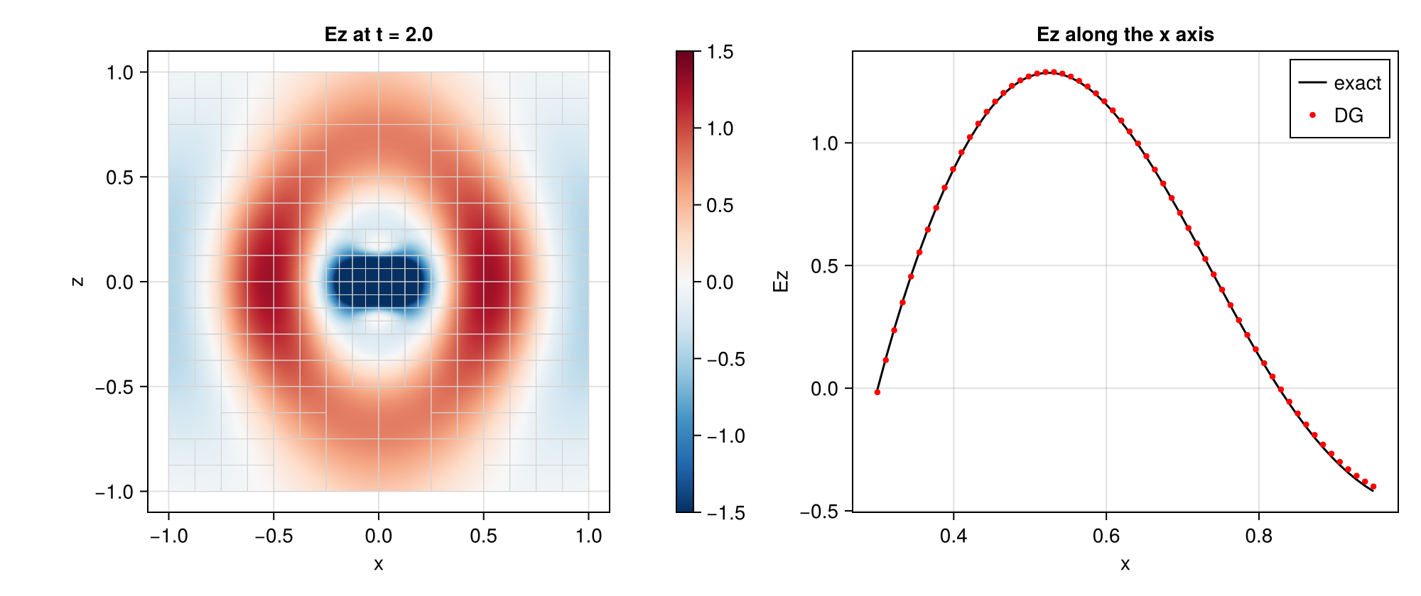
AMR is handled by Trixi's mesh and callbacks. The P4est dipole example combines a distance indicator around the source with an energy-gated wave indicator. The distance criterion retains resolution around the narrow source and the wave criterion follows the pulse.
Point interpolation and plotting geometry must be rebuilt after adaptation. The visualization sampler captures each live state together with its current mesh, rather than interpreting earlier solution vectors on the final mesh. See Figures and videos.
Adaptive P4est dipole example
Refinement is retained around the source and follows the pulse. The displayed mesh and numerical line probe are rebuilt together after adaptation.